So, maybe you have decided to get involved in this new Deep Learning wave of open source projects. The neural networks are kind of slow on a traditional computer. They have to do a lot of matrix math across thousands of neurons.
The traditional CPU is really a latency engine...run everything ASAP. The GPU, on the other hand, is a bandwidth engine. It may be slow getting started but it can far exceed the CPU in parallelism once its running. The typical consumer CPU is 4 cores + hyperthreading which gets you about 8 threads (virtual cores). Meanwhile, an entry level Pascal based GeForce 1050 will give you 768 CUDA cores. Very affordable and only 75 watts of power. You can go bigger but the smallest is huge compared to a CPU.
I've looked around the internet and haven't found good and complete instructions on how to setup for an Nvidia video card on a current version of Fedora. (The instructions at rpmfusion is misleading and old.) So, this post is dedicated to setting up a Fedora 25 system with a recent Nvidia card.
The Setup
With your old card installed and booted up...
1) Blacklist nouveau
# vi /etc/modprobe.d/disable-nouveau.conf
add the next line:
blacklist nouveau
2) Edit boot options
# vi /etc/default/grub
On the GRUB_CMDLINE_LINUX line
add: nomodeset
remove: rhgb
save, exit, and then run either
# grub2-mkconfig -o /boot/grub2/grub.cfg
Or if a UEFI system:
# grub2-mkconfig -o /boot/efi/EFI/<os>/grub.cfg
(Note: <os> should be replaced with redhat, centos, fedora as appropriate.)
3) Setup rpmfusion-nonfree:
# wget https://download1.rpmfusion.org/nonfree/fedora/rpmfusion-nonfree-release-25.noarch.rpm
# rpm -ivh rpmfusion-nonfree-release-25.noarch.rpm
4) Enable rpmfusion-nonfree
# vi /etc/yum.repos.d/rpmfusion-nonfree.repo
# vi /etc/yum.repos.d/rpmfusion-nonfree-updates.repo
In each, change to:
enabled=1
4) Update repos
# dnf --refresh check-update
See if new release package
# dnf update rpmfusion-nonfree-release.noarch
5) Start by getting rid of nouveau
# dnf remove xorg-x11-drv-nouveau
6) Install current nvidia drivers:
# dnf install xorg-x11-drv-nvidia-kmodsrc xorg-x11-drv-nvidia xorg-x11-drv-nvidia-libs xorg-x11-drv-nvidia-cuda akmod-nvidia kernel-devel akmod-nvidia --enablerepo=rpmfusion-nonfree-updates-testing
7) Install video accelerators:
# dnf install vdpauinfo libva-vdpau-driver libva-utils
8) Do any other system updates:
# dnf update
9) Shutdown and change out the video card. (Note that shutdown might take a few minutes as akmods is building you a new kernel module for your current kernel.) Reboot and cross your fingers.
Conclusion
This should get you up and running with video acceleration. This is not a CUDA environment for software development. That will require additional steps which involves registering and getting the Nvidia CUDA SDK. I'll leave that for another post when I get closer to doing AI experiments with the audit trail.
Friday, May 26, 2017
Thursday, May 25, 2017
Event overflow during boot
Today I wanted to explain something that I think needs to be corrected in the RHEL 7 DISA STIG. The DISA STIG is a Technical Guide that describes how to securely configure a system. I was looking through its recommendations and saw something in the audit section that ought to be fixed.
BOOT
When the Linux kernel is booted, there are some default values. One of those is the setting for the backlog limit. The backlog limit describes the size of the internal queue that holds events that are destined for the audit daemon. This queue is a holding area so that if the audit daemon is busy and can't get the event right away, they do not get lost. If this queue ever fills up all the way, then we have to make a decision about what to do. The options are ignore it, syslog that we dropped one, or panic the system. This is controlled by the '-f' option to auditctl.
Have you ever thought about the events in the system that are created before the audit daemon runs? Well, it turns out that when a boot is done with audit=1, then the queue is held until the audit daemon connects. After that happens, the audit daemon drains the queue and it functions normally. If the system does not boot with audit=1, then the events are sent to syslog immediately and are not held.
The backlog limit has a default setting of 64. This means that during boot if audit=1, then it will hold 64 records. Let's take a look at how this plays out in real life.
This is the event where the audit daemon started logging. In all likelihood the backlog limit got set during the same second. So, let's gather up a log like this:
The STIG calls for the backlog limit to be set to 8192. Assuming that we booted with the STIG suggested value, we can take a quick peek inside the csv file to see if 8192 is in the file. It is in my logs. If its not in yours, then increment the --end second by one and re-run. This assumes that you also have '-b 8192' in your audit rules.
What we want to do is create a stacked area graph that plots the cumulative number of events as one plot. This one shows events that are piling up in the backlog queue. We'll color this one red. Then we want to overlay that area graph with one that shows the size of the backlog queue. Its value will be 64 until the 8192 value comes along and then the size is expanded to 8192. We'll color this one blue.
The following R code creates our graph:
What this graph will tell us is if we are losing events. If we are not losing events, then the blue area will completely cover the red area. If we are losing events, then we will see some red. Everybody's system is different. You may have SE Linux AVCs or other things that happen which is different than mine. But for my system, I get the following chart:

Looking at it, we do see red area. Guestimating, it appears to drop about 50 events or so. This is clearly a problem if you wanted to have all of your events. So, what do you do about this?
There is another audit related kernel command line variable that you can set that initializes the backlog limit to something other than 64. If you wanted to match the number that the DISA STIG recommends, then on a grub2 system (such as rhel 7), you need to do the following as root:
That should do it.
Conclusion
The DISA STIG is a valuable resource in figuring out how to securely configure your Linux system. But there are places where it could be better. This blog shows that you can lose events if you don't take additional configuration steps to prevent this from happening. If you see "kauditd hold queue overflow" or something like that on your boot screen or in syslog, then be sure to set audit_backlog_limit on the kernel boot prompt.
BOOT
When the Linux kernel is booted, there are some default values. One of those is the setting for the backlog limit. The backlog limit describes the size of the internal queue that holds events that are destined for the audit daemon. This queue is a holding area so that if the audit daemon is busy and can't get the event right away, they do not get lost. If this queue ever fills up all the way, then we have to make a decision about what to do. The options are ignore it, syslog that we dropped one, or panic the system. This is controlled by the '-f' option to auditctl.
Have you ever thought about the events in the system that are created before the audit daemon runs? Well, it turns out that when a boot is done with audit=1, then the queue is held until the audit daemon connects. After that happens, the audit daemon drains the queue and it functions normally. If the system does not boot with audit=1, then the events are sent to syslog immediately and are not held.
The backlog limit has a default setting of 64. This means that during boot if audit=1, then it will hold 64 records. Let's take a look at how this plays out in real life.
$ ausearch --start boot --just-one
----
time->Wed May 24 06:55:20 2017
node=x2 type=DAEMON_START msg=audit(1495623320.378:4553): op=start ver=2.7.7 format=enriched kernel=4.10.15-200.fc25.x86_64 auid=4294967295 pid=863 uid=0 ses=4294967295 subj=system_u:system_r:auditd_t:s0 res=success
----
time->Wed May 24 06:55:20 2017
node=x2 type=DAEMON_START msg=audit(1495623320.378:4553): op=start ver=2.7.7 format=enriched kernel=4.10.15-200.fc25.x86_64 auid=4294967295 pid=863 uid=0 ses=4294967295 subj=system_u:system_r:auditd_t:s0 res=success
This is the event where the audit daemon started logging. In all likelihood the backlog limit got set during the same second. So, let's gather up a log like this:
ausearch --start boot --end 06:55:20 --format csv > ~/R/audit-data/audit.csv
The STIG calls for the backlog limit to be set to 8192. Assuming that we booted with the STIG suggested value, we can take a quick peek inside the csv file to see if 8192 is in the file. It is in my logs. If its not in yours, then increment the --end second by one and re-run. This assumes that you also have '-b 8192' in your audit rules.
What we want to do is create a stacked area graph that plots the cumulative number of events as one plot. This one shows events that are piling up in the backlog queue. We'll color this one red. Then we want to overlay that area graph with one that shows the size of the backlog queue. Its value will be 64 until the 8192 value comes along and then the size is expanded to 8192. We'll color this one blue.
The following R code creates our graph:
library(ggplot2)
# Read in the logs
audit <- read.csv("~/R/audit-data/audit.csv", header=TRUE)
# Create a running total of events
audit$total <- as.numeric(rownames(audit))
# create a column showing backlog size
# Default value is 64 until auditctl resizes it
# We choose a fill of 500 so the Y axiz doesn't make leakage too small
audit$backlog <- rep(64,nrow(audit))
audit$backlog[which(audit$OBJ_PRIME == 8192):nrow(audit)] = 500
# Now create a stacked area graph showing the leakage
plot1 = ggplot(data=audit) +
geom_area(fill = "red", aes(x=total, y=total, group=1)) +
geom_area(fill = "blue", aes(x=total, y=backlog, group=2)) +
labs(x="Event Number", y="Total")
print(plot1)
What this graph will tell us is if we are losing events. If we are not losing events, then the blue area will completely cover the red area. If we are losing events, then we will see some red. Everybody's system is different. You may have SE Linux AVCs or other things that happen which is different than mine. But for my system, I get the following chart:

Looking at it, we do see red area. Guestimating, it appears to drop about 50 events or so. This is clearly a problem if you wanted to have all of your events. So, what do you do about this?
There is another audit related kernel command line variable that you can set that initializes the backlog limit to something other than 64. If you wanted to match the number that the DISA STIG recommends, then on a grub2 system (such as rhel 7), you need to do the following as root:
- vi /etc/default/grub
- find "GRUB_CMDLINE_LINUX=" and add somewhere within the quotes and probably right after audit=1 audit_backlog_limit=8192. Save and exit.
- rebuild grub2 menu with: grub2-mkconfig -o /boot/grub2/grub.cfg. If UEFI system, then: grub2-mkconfig -o /boot/efi/EFI/<os>/grub.cfg (Note: <os> should be replaced with redhat, centos, fedora as appropriate.)
That should do it.
Conclusion
The DISA STIG is a valuable resource in figuring out how to securely configure your Linux system. But there are places where it could be better. This blog shows that you can lose events if you don't take additional configuration steps to prevent this from happening. If you see "kauditd hold queue overflow" or something like that on your boot screen or in syslog, then be sure to set audit_backlog_limit on the kernel boot prompt.
Tuesday, May 9, 2017
Day 1 at GTC 2017

This is a review of Day 1 of the Nvidia GTC 2017 Conference. Frankly, there is so much going on in GPU and Deep Learning as it relates to every industry, it's crazy...and its infectious. What I'm doing is looking down the road to the next steps for the audit system. What I'm investigating is how best to analyze the logs. How do you weed out the mundane normal system operation from the things that you had better pay attention to. Oh, and in real time. And at scale.
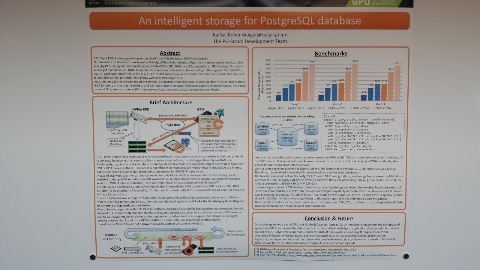
What I can tell you is I'm amazed at all the AI technology on display here. I took labs and built neural networks for data analysis. I can see the future of security situational awareness all around me but its in pieces needing to be assembled for a single purpose. I don't think I'll go too deep in this blog at what I'm seeing. But in the coming months I will be doing some experiments in applying different kinds of analysis to the audit trail. This will include looking at LSTMs, RNNs, and decision trees. What I'll do in this blog is just show you some posters that were in the main hall. All of these caught my eye for problems I'm currently thinking about.


Friday, May 5, 2017
Audit Record Fields Visualized
Before we move on from Dendrograms, I wanted to write about a post that combines what we have learned about the auparse library and R visualizations. Sometimes what you want to do requires writing a helper script that gets exactly the information you want. Then once we have prepared data, we can then take it through visualization. What I want to demonstrate in this post is how to create a graph of the audit record grammar.
Audit Records
The first step is to create a program based on auparse that will iterate over every event, and then over every record, and then over every field. We want to graph this by using a Dendrogram which means that things that are alike share common nodes and things that are different branch away. We want to label each record with its record type. Since we know that every record type is different, it would not be a good idea to start the line off with the record type. We will place it at the end just incase two records are identical except the record type.
Once our program is at the beginning of a record, we will iterate over every field and output its name. Since we know that we need a delimiter for the tree map, we can insert that at the time we create the output. Sound like a plan? Then go ahead and put this into fields-csv.c
Then compile it like:
Next, let's collect our audit data. We are absolutely going to have duplicate records. So, let's use the sort and uniq shell script tools to winnow out the duplicates.
Let's go into RStudio and turn this into a chart. If you feel you understand the dendrogram programming from the last post, go ahead and dive into it. The program, when finished, should be 6 actual lines of code. This program will has one additional problem that we have to solve.
The issue is that we did not actually create a normalized csv file where every record has the same number of fields. What R will do is normalize it so that all rows have the same number of columns. We don't want that. So, what we will do is use the gsub() function to trim the trailing slashes off. Other than that, you'll find the code remarkably similar to the previous blog post.
When I run the program, with my logs I get the following diagram. Its too big to paste into this blog, but just follow the link to see it full sized:
http://people.redhat.com/sgrubb/audit/record-fields.html
Conclusion
The Dendrogram is a useful tool to show similarity and structure of things. We were able to apply lessons from two previous blogs to produce something new. This can be applied in other ways where its simply easier to collect the right data and shape it during collection to make visualizing easier. Sometimes you may want to do data fusion at collection time to combine external information with the audit events and in that case you can do it at collection time of do an inner join like we did when creating sankey diagrams. Now, go write some neat tools.
Audit Records
The first step is to create a program based on auparse that will iterate over every event, and then over every record, and then over every field. We want to graph this by using a Dendrogram which means that things that are alike share common nodes and things that are different branch away. We want to label each record with its record type. Since we know that every record type is different, it would not be a good idea to start the line off with the record type. We will place it at the end just incase two records are identical except the record type.
Once our program is at the beginning of a record, we will iterate over every field and output its name. Since we know that we need a delimiter for the tree map, we can insert that at the time we create the output. Sound like a plan? Then go ahead and put this into fields-csv.c
#include <stdio.h>
#include <ctype.h>
#include <sys/stat.h>
#include <auparse.h>
static int is_pipe(int fd)
{
struct stat st;
if (fstat(fd, &st) == 0) {
if (S_ISFIFO(st.st_mode))
return 1;
}
return 0;
}
int main(int argc, char *argv[])
{
auparse_state_t *au;
if (is_pipe(0))
au = auparse_init(AUSOURCE_DESCRIPTOR, 0);
else if (argc == 2)
au = auparse_init(AUSOURCE_FILE, argv[1]);
else
au = auparse_init(AUSOURCE_LOGS, NULL);
if (au == NULL) {
printf("Failed to access audit material\n");
return 1;
}
auparse_first_record(au);
do {
do {
int count = 0;
char buf[32];
const char *type = auparse_get_type_name(au);
if (type == NULL) {
snprintf(buf, sizeof(buf), "%d",
auparse_get_type(au));
type = buf;
}
do {
const char *name;
count++;
if (count == 1)
continue;
name = auparse_get_field_name(au);
if (name[0] == 'a' && isdigit(name[1]))
continue;
if (count == 2)
printf("%s", name);
else
printf(",%s", name);
} while (auparse_next_field(au) > 0);
printf(",%s\n", type);>
} while (auparse_next_record(au) > 0);
} while (auparse_next_event(au) > 0);
auparse_destroy(au);
return 0;
}
Then compile it like:
gcc -o fields-csv fields-csv.c -lauparse
Next, let's collect our audit data. We are absolutely going to have duplicate records. So, let's use the sort and uniq shell script tools to winnow out the duplicates.
ausearch --start this-year --raw | ./fields-csv | sort | uniq > ~/R/audit-data/year.csv
Let's go into RStudio and turn this into a chart. If you feel you understand the dendrogram programming from the last post, go ahead and dive into it. The program, when finished, should be 6 actual lines of code. This program will has one additional problem that we have to solve.
The issue is that we did not actually create a normalized csv file where every record has the same number of fields. What R will do is normalize it so that all rows have the same number of columns. We don't want that. So, what we will do is use the gsub() function to trim the trailing slashes off. Other than that, you'll find the code remarkably similar to the previous blog post.
library(data.tree)
library(networkD3)
# Load in the data
a <- read.csv("~/R/audit-data/year.csv", header=FALSE, stringsAsFactors = FALSE)
# Create a / separated string list which maps the fields
a$pathString <- do.call(paste, c("record", sep="/", a))
# Previous step normalized the path based on record with most fields.
# Need to remove trailing '/' to fix it.
gsub('/+$', '', a$pathString)
# Now convert to tree structure
l <- as.Node(a, pathDelimiter = "/")
# And now as a hierarchial list
b <- ToListExplicit(l, unname = TRUE)
# And visualize it
diagonalNetwork(List = b, fontSize = 12, linkColour = "black", height = 4500, width = 2200)
When I run the program, with my logs I get the following diagram. Its too big to paste into this blog, but just follow the link to see it full sized:
http://people.redhat.com/sgrubb/audit/record-fields.html
Conclusion
The Dendrogram is a useful tool to show similarity and structure of things. We were able to apply lessons from two previous blogs to produce something new. This can be applied in other ways where its simply easier to collect the right data and shape it during collection to make visualizing easier. Sometimes you may want to do data fusion at collection time to combine external information with the audit events and in that case you can do it at collection time of do an inner join like we did when creating sankey diagrams. Now, go write some neat tools.
Thursday, May 4, 2017
Dendrograms
In this post we will resume our exploration of data science by learning a new kind of visualization technique. Sometimes we need to show exact relationships that naturally fall out as a tree. You have a root and branches that show how something is similar and then how it becomes different as you know more. This kind of diagram is known as a Dendrogram.
I See Trees
The linux file system is a great introductory data structure that lends itself to being drawn as a tree because...it is. You have a root directory and then subdirectories and then subdirectories under those. Turning this into a program that draws your directory structure is remarkably simple. First, let's collect some data to explore. I want to choose the directories under the /usr directory but not too many. So, run the following command:
OK. We have our data. It turns out that there is a package in R that is a perfect fit for this kind of data. Its called data.tree. If you do not have that installed into RStudio, go ahead and run
The way that this package works is that it wants to see things represented as a string separated by a delimiter. It wants this mapping to be under a column called pathString. So, this is why we created the CSV file the way we did. The paths found by the find command have '/' as a delimiter. So, this makes our program dead simple:
On my system you get a picture something like this:

Programming in R is a lot like cheating. (Quote me on that.) Four actual lines of code to produce this. How many lines of C code would it take to do this? We can see grouping of how things are similar by how many nodes they share. Something that is very different branches away on the first node. Things that are closely related share many of the same nodes.
So, lets use this to visualize how closely related some audit events are. Let's collect some audit data:
What we want to do with this is fashion the data into the same layout that we had with the directory paths. The audit data has 15 columns. To show how events are related to one another we only want the EVENT_KIND and the EVENT columns. So our first step is to create a new dataframe with just those. Next we need to take each row and turn it into a string that has each column delimited by some character. We'll choose '/' again to keep it simple. But this time we need to create our own pathString column and fill it with the string. We will use the paste function to glue it altogether. And the rest of the program is just like the previous one.
With my audit logs, I get a picture like this:

You can clearly see the grouping of events that are related to a user login, events related to system services, and Mandatory Access Control (mac) events among others. You can try this on bigger data sets.
So let's do one last dendrogram and call it a day. Using the same audit csv file, suppose you wanted to show user, user session, time of day, and action, can you guess how to do it? Look at the above program. You only have to change 2 lines. Can you guess which ones?
Here they are:
Which yields a picture like this from my data:

Conclusion
The dendrogram is a good diagram to show how things are alike and how they differ. Events tend to differ based on time and this can be useful in showing order of time series data. Creating a dendrogram is dead simple and is typically 6 lines of actual code. This adds one more tool to our toolbox for exploring security data.
I See Trees
The linux file system is a great introductory data structure that lends itself to being drawn as a tree because...it is. You have a root directory and then subdirectories and then subdirectories under those. Turning this into a program that draws your directory structure is remarkably simple. First, let's collect some data to explore. I want to choose the directories under the /usr directory but not too many. So, run the following command:
[sgrubb@x2 dendrogram]$ echo "pathString" > ~/R/audit-data/dirs.csv
[sgrubb@x2 dendrogram]$ find /usr -type d | head -20 >> ~/R/audit-data/dirs.csv
[sgrubb@x2 dendrogram]$ cat ~/R/audit-data/dirs.csv
pathString
/usr
/usr/bin
/usr/games
/usr/lib64
/usr/lib64/openvpn
/usr/lib64/openvpn/plugins
/usr/lib64/perl5
/usr/lib64/perl5/PerlIO
/usr/lib64/perl5/machine
/usr/lib64/perl5/vendor_perl
/usr/lib64/perl5/vendor_perl/Compress
/usr/lib64/perl5/vendor_perl/Compress/Raw
/usr/lib64/perl5/vendor_perl/threads
/usr/lib64/perl5/vendor_perl/Params
/usr/lib64/perl5/vendor_perl/Params/Validate
/usr/lib64/perl5/vendor_perl/Digest
/usr/lib64/perl5/vendor_perl/MIME
/usr/lib64/perl5/vendor_perl/Net
/usr/lib64/perl5/vendor_perl/Net/SSLeay
/usr/lib64/perl5/vendor_perl/Scalar
OK. We have our data. It turns out that there is a package in R that is a perfect fit for this kind of data. Its called data.tree. If you do not have that installed into RStudio, go ahead and run
install.packages("data.tree")
The way that this package works is that it wants to see things represented as a string separated by a delimiter. It wants this mapping to be under a column called pathString. So, this is why we created the CSV file the way we did. The paths found by the find command have '/' as a delimiter. So, this makes our program dead simple:
library(data.tree)
library(networkD3)
# Read in the paths
f <- read.csv("~/R/audit-data/dirs.csv", header=TRUE)
# Now convert to tree structure
l <- as.Node(f, pathDelimiter = "/")
# And now as a hierarchial list
b <- ToListExplicit(l, unname = TRUE)
# And visualize it
diagonalNetwork(List = b, fontSize = 10)
library(networkD3)
# Read in the paths
f <- read.csv("~/R/audit-data/dirs.csv", header=TRUE)
# Now convert to tree structure
l <- as.Node(f, pathDelimiter = "/")
# And now as a hierarchial list
b <- ToListExplicit(l, unname = TRUE)
# And visualize it
diagonalNetwork(List = b, fontSize = 10)
On my system you get a picture something like this:
Programming in R is a lot like cheating. (Quote me on that.) Four actual lines of code to produce this. How many lines of C code would it take to do this? We can see grouping of how things are similar by how many nodes they share. Something that is very different branches away on the first node. Things that are closely related share many of the same nodes.
So, lets use this to visualize how closely related some audit events are. Let's collect some audit data:
ausearch --start today --format csv > ~/R/audit-data/audit.csv
What we want to do with this is fashion the data into the same layout that we had with the directory paths. The audit data has 15 columns. To show how events are related to one another we only want the EVENT_KIND and the EVENT columns. So our first step is to create a new dataframe with just those. Next we need to take each row and turn it into a string that has each column delimited by some character. We'll choose '/' again to keep it simple. But this time we need to create our own pathString column and fill it with the string. We will use the paste function to glue it altogether. And the rest of the program is just like the previous one.
library(data.tree)
library(networkD3)
audit <- read.csv("~/R/audit-data/audit.csv", header=TRUE)
# Subset to the fields we need
a <- audit[, c("EVENT_KIND", "EVENT")]
# Prepare to convert from data frame to tree structure by making a map
a$pathString <- paste("report", a$EVENT_KIND, a$EVENT, sep="/")
# Now convert to tree structure
l <- as.Node(a, pathDelimiter = "/")
# And now as a hierarchial list
b <- ToListExplicit(l, unname = TRUE)
# And visualize it
diagonalNetwork(List = b, fontSize = 10)
With my audit logs, I get a picture like this:
You can clearly see the grouping of events that are related to a user login, events related to system services, and Mandatory Access Control (mac) events among others. You can try this on bigger data sets.
So let's do one last dendrogram and call it a day. Using the same audit csv file, suppose you wanted to show user, user session, time of day, and action, can you guess how to do it? Look at the above program. You only have to change 2 lines. Can you guess which ones?
Here they are:
a <- audit[, c("SUBJ_PRIME", "SESSION", "TIME", "ACTION")]
a$pathString <- paste("report", a$SUBJ_PRIME, a$SESSION, a$TIME, a$ACTION, sep="/")
a$pathString <- paste("report", a$SUBJ_PRIME, a$SESSION, a$TIME, a$ACTION, sep="/")
Which yields a picture like this from my data:
Conclusion
The dendrogram is a good diagram to show how things are alike and how they differ. Events tend to differ based on time and this can be useful in showing order of time series data. Creating a dendrogram is dead simple and is typically 6 lines of actual code. This adds one more tool to our toolbox for exploring security data.
Monday, May 1, 2017
Updating R
Its been a while since we talked about R. There is one important point that I wanted to raise since this is a security blog. That is that R and its packages must be updated just like any other package on your Linux system.
How To Update
The R packages use things like curl to pull remote content and thus need maintaining as curl is updated to fix its own CVE's. Some of the R packages are very complex and have several layers of dependencies and pull a lot of source code to recompile. I'll show you the easy way to fix all this.
First, start up Rstudio. Then find the menu item "Tools" and click on it. You will see a menu item that says "Check for package updates".

Click on it and it will "think" for a couple seconds while its fetching update information and comparing with your local repository. When its done, the dialog box will look something like this.

Then you click on "Select All" and then "Install updates" and it will start downloading source. It will recompile the R packages and install them to the runtime R repository off of your home directory. When it finishes, you are done. You can restart Rstudio to reload the packages with new ones and go back to doing data science things.
Conclusion
Its really simple to keep R updated. It has vulnerable packages just like anything else on your system. Occasionally there are feature enhancements. The hardest part is just developing the habit to update R periodically.
How To Update
The R packages use things like curl to pull remote content and thus need maintaining as curl is updated to fix its own CVE's. Some of the R packages are very complex and have several layers of dependencies and pull a lot of source code to recompile. I'll show you the easy way to fix all this.
First, start up Rstudio. Then find the menu item "Tools" and click on it. You will see a menu item that says "Check for package updates".
Click on it and it will "think" for a couple seconds while its fetching update information and comparing with your local repository. When its done, the dialog box will look something like this.
Then you click on "Select All" and then "Install updates" and it will start downloading source. It will recompile the R packages and install them to the runtime R repository off of your home directory. When it finishes, you are done. You can restart Rstudio to reload the packages with new ones and go back to doing data science things.
Conclusion
Its really simple to keep R updated. It has vulnerable packages just like anything else on your system. Occasionally there are feature enhancements. The hardest part is just developing the habit to update R periodically.
Subscribe to:
Posts (Atom)